Meta-analytic Death Match : dumb algebra guy v.s. the Bayesian King Kong

Maybe I overdid it with the title, but I think the data speak for themselves in the (?much) anticipated,  pre-announced comparison between a naive, algebra based solution and the Bayesian, Monte Carlo based one.

To carry out this comparison, I assumed:

• a large number of log-relative risks (big truths, )
• a large number of standard errors ()

and then

1. calculated the associated RR, 95% CI and p-values,
2. rounded the results down to two significant digits (3 for the p-value) to accommodate the most common set of requirements for reporting clinical research results
3. presented these to both approaches and compared the resulting estimates.

Simulations were carried over a wide range of (in the range of -0.8 to 0.8, corresponding to  RR of 2.24 and 0.45 (rounded to 2 significant figures!) which are typical estimates for many of the (well conducted) clinical studies in the literature. Standard errors were allowed to vary independently in the range of 0.1 to 3, yielding Signal to Noise Ratios () in the range of 0.27  to 8 (for those of you more comfortable with p-values, these SNRs correspond to 0.79 and 0.000000000000001 respectively).

To compare the two approaches against each other I calculated the following straightforward metrics:

1. the average squared difference ( Mean Square Error) between each algorithm estimate for   and the “truth” for each simulated pair of values ()
2. the MSE for the estimate

Considered in isolation these metrics may not entirely reflect the impact of  rounding on information loss and the ability of each of the 2 approaches considered to recover some of that loss. Furthermore, how can one arbitrate between the 2 algorithms if one had a larger MSE for but a smaller MSE for compared to the other? One possibility is to take the square root of the sum of the two MSEs (RMSE) which can be given a nice geometric interpretation (see below). Another possibility is to calculate information theory metrics (Kullback-Leibler divergence) between the distribution implied by the estimates of each algorithm and the original distribution (a Normal distribution with mean equal to and standard deviation equal to ). Such metrics can correspond to “distances” between the informational content of two distributions when the latter differ in one or more parameters.  Since the ultimate goal of both of these algorithms is to provide summary estimates for use in downstream meta-analysis (or other evidence synthesis endeavors), information theory metrics seem the most natural measures to use when contrasting different approaches to de-noising rounded numerical figures.

The results of the deathmatch are shown below:

In this figure the y-axis is the difference between the estimated – simulated logRR and the x-axis is the corresponding figure for the standard error. Hence, points closer to the center of the figure correspond to more accurate (less biased estimates). As one may observe, the overall spread of the estimates is much smaller for the Bayesian estimate than the one made by the simple Algebraic algorithm. This is reflected in the RMSE, which in this case can be given a geometric interpretation as the distance of each point from the center of the graph; for the Bayesian estimator it is  , while it is for the Algebraic one.

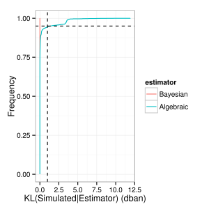
Switching over to the KL metric (measured in decibans i.e. tenths of the decimal logarithm) we see a similar pattern:

The Bayesian estimator outperforms the simple Algebraic one, but not by much: in only 5% of the cases (dashed horizontal line) does the difference between the simulated and the estimated distribution  is larger than 1 deciban (dashed vertical line), the smallest difference that one would be compelled to say that there is a meaningful difference between  two distributions.

Does this difference matter? The answer to this question is (as always) to the eyes of the beholder: if the difference between the two estimators is such as to push the results of a downstream evidence synthesis endeavour to the left (or right) of the mystical 0.05 p-value “hairline”, then this difference does matter (possibly a lot!). However for less “mission-critical” applications, the (not so) dumb Algebra solution maybe as good, and potentially more useful, for people who do not want to be programming their Monte Carlo samplers. As I already have programmed mine, I will be sticking with the Bayesian solution 🙂